PO Time and Space Complexity

Complexity Analysis

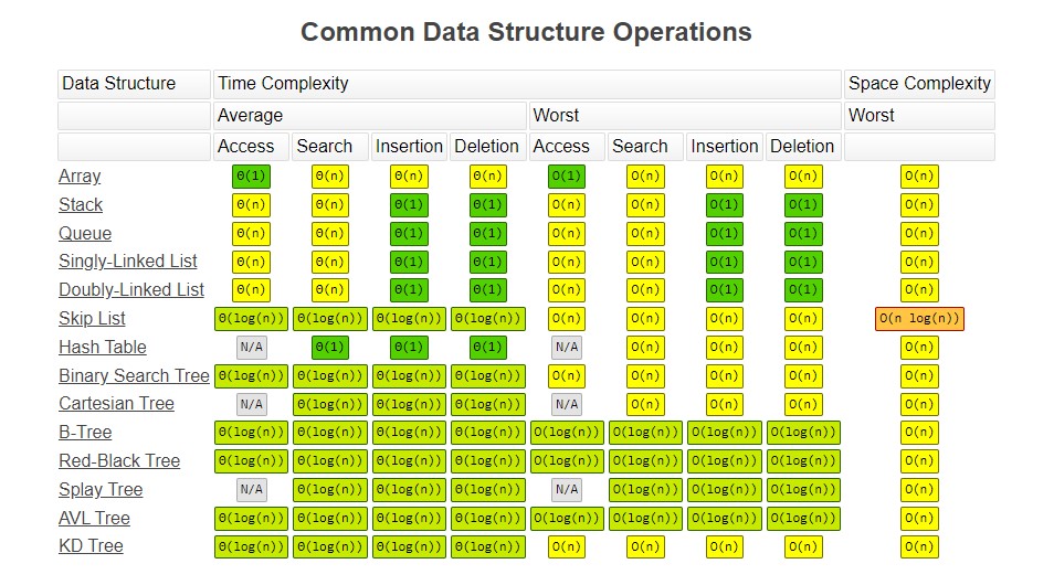
The process of determining how efficient an algorithm is. Complexity analysis involves finding both the time complexity and the space complexity of an algorithm, and is used to compare algorithms and determine whether one is better suited to a problem than another.

Time Complexity

A measure of how the runtime of an algorithm grows as the size of the input increases. It is expressed using Big O notation.

Note: Time Complexity ≠ Time taken. Time complexity is a rate of growth — it tells you how an algorithm scales, not how many milliseconds it takes on a specific machine.

Space Complexity

A measure of how much auxiliary (extra) memory an algorithm uses as the input size grows. It is expressed using Big O notation.

Note that space complexity counts additional space beyond the input itself — the input is already given and doesn't count against the algorithm's space usage in most analyses.

What is Big O Notation?

The notation used to describe the time complexity and space complexity of algorithms.

Variables used in Big O notation denote the sizes of inputs to algorithms.

For example, O(n) might be the time complexity of an algorithm that traverses through an array of length n; similarly, O(n + m) might be the complexity of an algorithm that traverses through an array of length n and a string of length m.

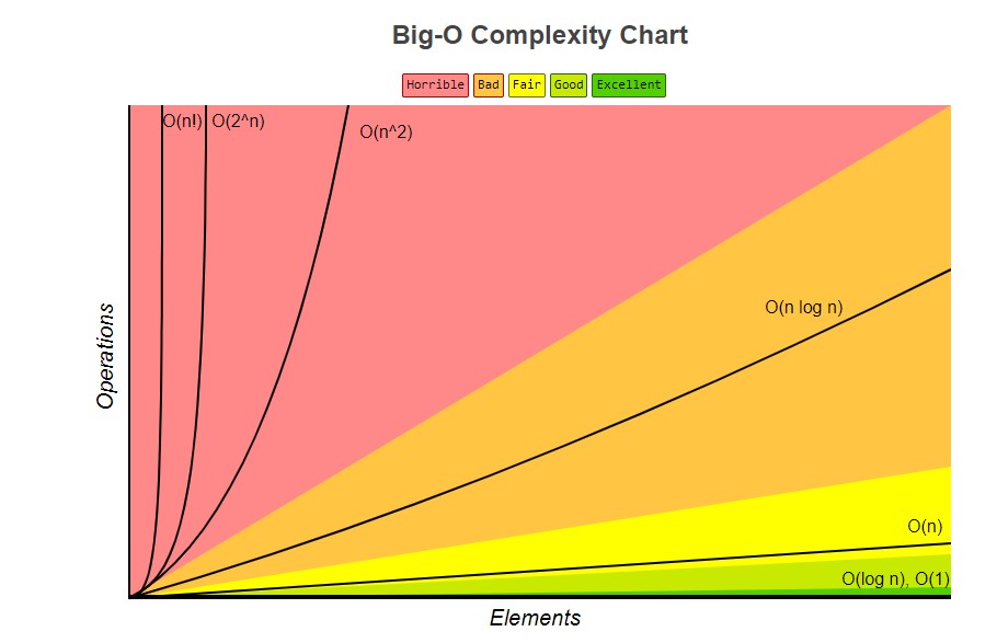
The following are common complexities and their Big O notations, ordered from fastest to slowest:

Constant: O(1)
Logarithmic: O(log n)
Linear: O(n)
Log-linear: O(n log n)
Quadratic: O(n²)
Cubic: O(n³)
Exponential: O(2ⁿ)
Factorial: O(n!)

Note: Always drop less dominant terms when expressing Big O. For example, O(n³ + log n) simplifies to O(n³), because for large n, the n³ term dominates completely and the log n term is negligible by comparison. Similarly, always drop constant coefficients: O(3n) = O(n).

screenshot of the app

Notations Used in Complexity Analysis

Omega (Ω) — Lower Bound

Omega notation gives the lower bound on the running time of an algorithm. It means the algorithm will take at least this long (in the best case). For example, Ω(n) means the algorithm always does at least linear work regardless of input.
Big O (O) — Upper Bound

Big O notation gives the upper bound on the running time. It means the algorithm will take at most this long (in the worst case). This is the most commonly used notation in practice because worst-case guarantees are what matter most for production systems.
Theta (Θ) — Tight Bound

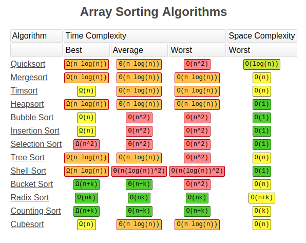
Theta notation means the lower and upper bounds are the same — the algorithm's runtime grows exactly at this rate (within constant factors) for all large inputs. For example, Θ(n log n) means the algorithm's runtime is both O(n log n) and Ω(n log n).

In everyday conversation, people often use "Big O" loosely when they technically mean Theta. Merge sort is Θ(n log n) in all cases — its best, average, and worst case are all n log n — whereas quicksort is O(n log n) on average but O(n²) in the worst case.

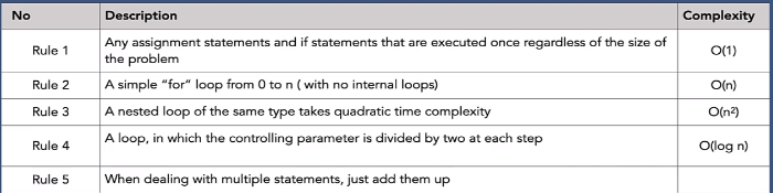
How to Measure Code Using Big O?

screenshot of the app

Space Complexity Examples

package com.praveen.complexity;

public class SpaceComplexityExamples {

    // Space: O(1)
    // Only a fixed number of scalar variables (sum, i) regardless of input size
    public static int example1(int n) {
        int sum = 0;
        for (int i = 1; i <= n; i++) {
            sum += i;
        }
        return sum;
    }

    // Space: O(n)
    // Allocates a result array of size 2*n — grows linearly with input
    public static int[] example2(int[] array) {
        int n = array.length;
        int[] result = new int[2 * n];
        for (int i = 0; i < n; i++) {
            result[i] = array[i];
            result[n + i] = array[i];
        }
        return result;
    }

    // Space: O(n)  ← corrected from O(n*m)
    // The matrix is the INPUT (not counted against auxiliary space).
    // The only auxiliary allocation is `int[] array = new int[n]` — size n.
    // The sum variable is O(1). So total auxiliary space is O(n), not O(n*m).
    public static int example3(int[][] matrix) {
        int n = matrix.length;
        int m = matrix[0].length;
        int sum = 0;
        for (int i = 0; i < n; i++) {
            for (int j = 0; j < m; j++) {
                sum += matrix[i][j];
            }
        }
        int[] array = new int[n];
        for (int i = 0; i < n; i++) {
            array[i] = matrix[i][0];
        }
        return sum;
    }
}

Time Complexity Examples

package com.praveen.complexity;

public class TimeComplexityExamples {

    // Time: O(n²)
    // Two nested loops each running up to n iterations
    public static boolean hasDuplicates(int[] array) {
        int n = array.length;
        for (int i = 0; i < n; i++) {
            for (int j = 0; j < n; j++) {
                if (i != j && array[i] == array[j]) {
                    return true;
                }
            }
        }
        return false;
    }

    // Time: O(n²)
    // The dominant term is the nested loop: n*(n+1)/2 iterations = O(n²).
    // The two subsequent single loops are O(n) and O(1) — both negligible.
    public static int f(int n) {
        int sum = 0;
        for (int i = 1; i <= n; i++) {
            for (int j = 1; j <= i; j++) {
                sum += i * j;
            }
        }
        for (int i = 0; i < n; i++) {
            sum = sum - i;
        }
        for (int i = 0; i < 100; i++) {
            sum += i;
        }
        return sum;
    }

    // Time: O(n + m)
    // One pass through A (n elements), one pass through B (m elements)
    public static int[] union(int[] A, int[] B) {
        int n = A.length;
        int m = B.length;
        int[] C = new int[n + m];
        int index = 0;
        for (int i = 0; i < n; i++) {
            C[index] = A[i];
            index++;
        }
        for (int i = 0; i < m; i++) {
            C[index] = B[i];
            index++;
        }
        return C;
    }

    // Time: O(n * m)
    // Two nested loops: outer runs n times, inner runs m times per outer iteration
    public static int matrixSum(int[][] matrix) {
        int n = matrix.length;
        int m = matrix[0].length;
        int sum = 0;
        for (int i = 0; i < n; i++) {
            for (int j = 0; j < m; j++) {
                sum += matrix[i][j];
            }
        }
        return sum;
    }

    // Time: O(log n)
    // i is halved on every iteration: n → n/2 → n/4 → ... → 1
    // The number of iterations is log₂(n)
    public static int g(int n) {
        int result = 0;
        int i = n;
        while (i > 1) {
            result += i;
            i /= 2;
        }
        return result;
    }
}

DSA Course

Time and Space Complexity