Back to DSA Course

Data Structure

What is a Data Structure?

A data structure is a way of defining, storing, and retrieving data in a structured and systematic way. A data structure may contain different types of data items.

The Need for Data Structures

As the amount of data grows rapidly and applications become more complex, the following problems arise:

• Processing Speed: As data volumes increase, high-speed processing is required to handle massive amounts of data efficiently. A poor choice of data structure can make an otherwise fast algorithm unworkably slow.
• Searching Data: Consider an inventory with 200 items. If your application searches for a particular item by scanning every entry every time, it traverses all 200 items on every search. The right data structure (e.g., a hash table or a balanced BST) can reduce this to O(1) or O(log n).
• Multiple Concurrent Requests: Millions of users simultaneously querying a web server need efficient data organization so the server can serve them without becoming a bottleneck.

Advantages of Data Structures

• Efficiency: The right data structure reduces both time complexity and space complexity, allowing an application to handle larger data volumes with the same hardware.
• Reusability: Once a data structure is implemented and tested, it can be used across many parts of an application. Java's Collections Framework is exactly this — a library of proven, reusable data structures.
• Abstraction: Abstract Data Types (ADTs) define what operations a data structure supports without exposing how they are implemented. Clients depend on the interface (e.g., List, Queue, Map), not the implementation (ArrayList, LinkedList, HashMap).

Types of Data Structures

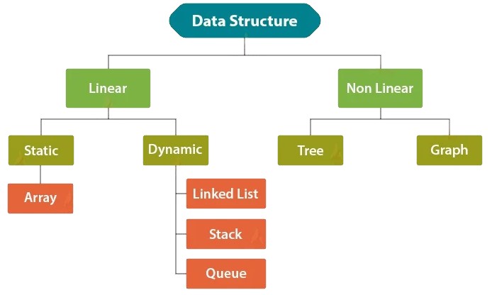
1. Linear Data Structures

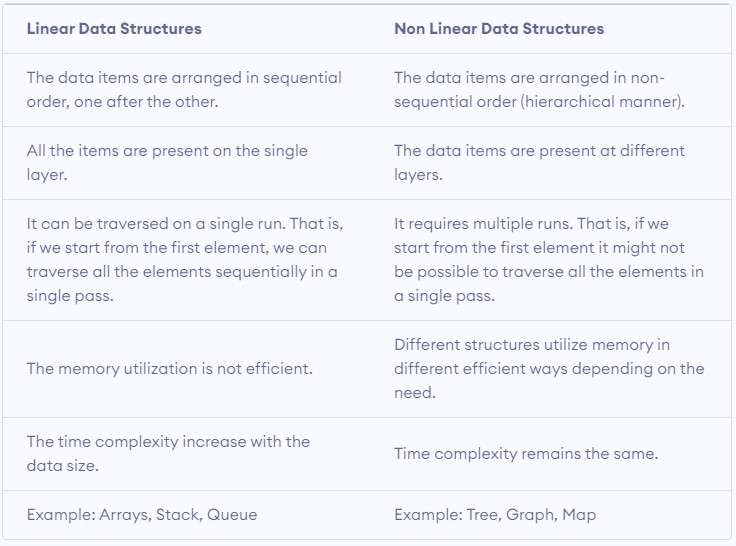
In linear data structures, elements are arranged sequentially, one after the other. Because elements follow a particular order, they are straightforward to implement and traverse.

However, for problems where the access pattern is not sequential — or where elements have hierarchical or network relationships — linear structures may not be the best choice.

• Array: Elements stored in contiguous memory locations. All elements are of the same type. Supports O(1) random access by index but O(n) insertion/deletion in the middle.

• Stack: Follows the LIFO (Last-In, First-Out) principle. The last element added is the first one removed — like a pile of plates where you always take from the top. Use cases: function call stack, undo/redo, expression evaluation.

• Queue: Follows the FIFO (First-In, First-Out) principle. The first element added is the first one removed — like a ticket queue. Use cases: task scheduling, breadth-first search, message buffers.

• Linked List: Elements (nodes) are connected through pointers. Each node stores data and the address of the next node. Supports O(1) insertion/deletion at the head but O(n) random access.

2. Non-Linear Data Structures

In non-linear data structures, elements are not in any sequence. Instead, they are arranged hierarchically or in a network, where one element may be connected to one or more others.

• Graph: Each entity is represented as a vertex (node), and relationships between entities are represented as edges. Graphs can be directed or undirected, weighted or unweighted. Use cases: social networks, maps, dependency graphs.

• Tree: A special case of a graph — a connected, acyclic graph. There is exactly one path between any two nodes. In a rooted tree, one node is designated as the root, and all others are reachable from it through parent-child edges. Use cases: file systems, HTML DOM, expression trees, binary search trees, heaps.

Linear vs. Non-Linear Data Structures

Data Structure Operations

• Insertion: Add a new data element to the data structure.
• Deletion: Remove a data element from the data structure.
• Sorting: Rearrange data in increasing or decreasing order.
• Searching: Find the location of a specific data element.
• Merging: Combine the elements of two sorted structures into a single sorted structure.
• Traversal: Visit each data element exactly once. Different data structures support different traversal orders (e.g., in-order, pre-order, post-order for trees; BFS/DFS for graphs).

---

Algorithm

What is an Algorithm?

An algorithm is a step-by-step procedure that defines a finite set of instructions to be executed in a specific order to achieve a desired output for a given input.

An algorithm must be:

• Correct: Produces the right output for all valid inputs.
• Finite: Terminates after a finite number of steps.
• Unambiguous: Each step is clearly defined with no room for interpretation.
• Efficient: Uses time and space resources proportionally.

Why Algorithms Matter

• Gives a model of running time and space requirements before writing code.
• Helps decide what hardware is needed to handle expected data volumes.
• Distinguishes between what is computationally feasible and what is not.
• Algorithmic improvements are often more impactful than hardware improvements — an O(n log n) algorithm beats an O(n²) algorithm regardless of how fast the hardware is.

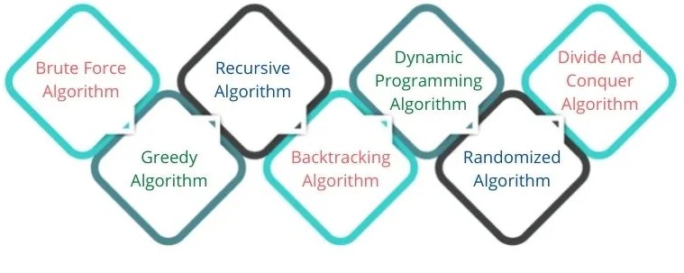
Types of Algorithms

• Brute Force: Try all possibilities exhaustively until a solution is found. Guarantees finding the optimal solution if one exists, but is typically too slow for large inputs. Example: checking all possible subsets to find the one with the maximum sum.

• Recursive: Solve a problem by breaking it into smaller subproblems of the same type, solving each recursively, and combining the results. Requires a base case that stops the recursion. Examples: merge sort, tree traversal, factorial.

• Dynamic Programming: Solve problems by breaking them into overlapping subproblems and storing (memoizing or tabulating) the result of each subproblem to avoid recomputing it. Best applied when a problem has optimal substructure and overlapping subproblems. Examples: Fibonacci, longest common subsequence, knapsack.

  Dynamic Programming is not just "memoization" — the two approaches (top-down with memoization, bottom-up with tabulation) are both DP. The key insight is that you're trading space for time by caching results.

• Divide and Conquer: Divide the problem into independent subproblems, solve each recursively, then combine results. Unlike DP, subproblems do not overlap. Examples: merge sort, quick sort, binary search.

• Greedy: Build the solution one step at a time, always making the locally optimal choice at each step, hoping it leads to a globally optimal solution. Greedy works when the problem has the greedy-choice property — not all optimization problems do. Examples: Huffman encoding, Dijkstra's shortest path (with non-negative weights), activity selection.

• Backtracking: Explore all candidate solutions by incrementally building candidates, and abandon ("backtrack") a candidate as soon as it is determined it cannot lead to a valid solution. More intelligent than brute force because it prunes the search space. Examples: N-Queens, Sudoku solver, subset sum.

• Randomized: Use random numbers in the algorithm's logic to make decisions. Can provide good average-case performance even when worst-case is poor. Examples: randomized quicksort (random pivot selection), Monte Carlo algorithms.

---

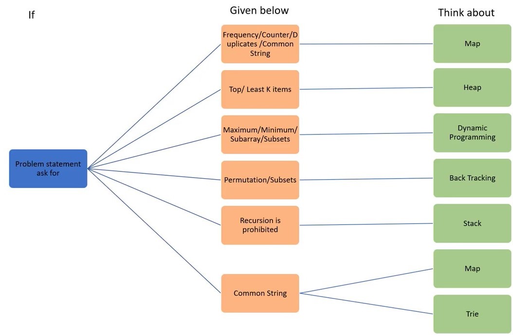
Mindmap for Coding Interviews